| 일 | 월 | 화 | 수 | 목 | 금 | 토 |
|---|---|---|---|---|---|---|
| 1 | 2 | 3 | 4 | 5 | ||
| 6 | 7 | 8 | 9 | 10 | 11 | 12 |
| 13 | 14 | 15 | 16 | 17 | 18 | 19 |
| 20 | 21 | 22 | 23 | 24 | 25 | 26 |
| 27 | 28 | 29 | 30 |
- 인공지능학원
- 유투브크롤링
- 광주인공지능학원
- python
- DataFrame
- iris붓꽃
- 과대적합제어
- relu
- tfidf
- 셀리니움
- sellenium
- 웹크롤링
- 딥러닝
- CountVectorizer
- 파이썬
- 인공지능
- 데이터프레임
- servlet
- 크롤링
- Selenium
- 댓글분석
- 활성화함수
- 스마트인재개발원
- permisision부여
- 머신러닝
- 광주국비지원학원
- 토큰화
- 과대적합
- 자바
- jsp
- Today
- Total
+ Hello +
[광주인공지능학원] CNN 개, 고양이 분류 본문
안녕하세요 !
이번주는 광주인공지능학원 스마트개발원에서
CNN을 통해 개, 고양이 사진을 분류하는 방법에 대해 배웠답니다!
밑의 자료는 광주인공지능학원에서 제공받은 수업 자료를 토대로 작성하였습니다.
- 먼저 jupyter 실행 폴더에 개, 고양이 사진 폴더 집어넣기
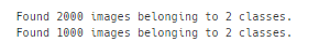
* 데이터 구성 살펴보기
- 총 3000개 (train 2000장, validation 1000장)로 구성된 데이터 셋
- 각각의 데이터는 절반은 개 사진(1000장 500장) 절반은 고양이 사진(1000장 500장)
- 강아지 고양이 사진 불러오기
- train, test, validation
train_dir = './dogs_vs_cats_small/train'
test_dir =  './dogs_vs_cats_small/test'

train_dogs_dir ='./dogs_vs_cats_small/train/dogs'
train_cats_dir ='./dogs_vs_cats_small/train/cats'

test_dogs_dir =  './dogs_vs_cats_small/test/dogs'
test_cats_dir =  './dogs_vs_cats_small/test/cats'

validation_dogs_dir =  './dogs_vs_cats_small/validation/dogs'
validation_cats_dir ='./dogs_vs_cats_small/validation/cats'
- listdir() : 해당 폴더에 있는 파일을 가져온다
print("훈련 개 데이터 수 : {}".format(len(os.listdir(train_dogs_dir))))
print("훈련 고양이 데이터 수 : {}".format(len(os.listdir(train_cats_dir))))
print("테스트 개 데이터 수 : {}".format(len(os.listdir(test_dogs_dir))))
print("테스트 고양이 데이터 수 : {}".format(len(os.listdir(test_cats_dir))))
print("검증 개 데이터 수 : {}".format(len(os.listdir(validation_dogs_dir))))
print("검증 고양이 데이터 수 : {}".format(len(os.listdir(validation_cats_dir))))
* 이미지 전처리
- 이미지를 같은 크기로 만들어주어야함
- 0 ~ 255 범위의 픽셀값을 0 ~ 1 사이의 범위로 변환 -> 분산 감소
- 라벨링
- ImageDataGenerator() 함수 사용해서 처리
- flow_from_directory():폴더에서 이미지 가져오기
- 이진분류 : binary
- 다중분류 : categorical
- 라벨 번호는 0부터 시작
- 폴더는 알파벳 순으로 읽음
from tensorflow.keras.preprocessing.image import ImageDataGenerator

# 픽셀값을 0 ~ 1 사이로 변환
train_gen = ImageDataGenerator(rescale = 1./255)
test_gen = ImageDataGenerator(rescale = 1./255)

# 폴더명, 이미지크기, 한 번에 변환할 이미지 수, 라벨링 모드
train_generator = train_gen.flow_from_directory(train_dir,
                                                target_size=(150,150),
                                                batch_size = 50,
                                                 class_mode = 'binary'
                                                )
test_generator = train_gen.flow_from_directory(test_dir,
                                                target_size=(150,150),
                                                batch_size = 50,
                                                 class_mode = 'binary'
                                                )
- 라벨링 결과 확인하기
print(train_generator.class_indices)
print(test_generator.class_indices)
- 초기화를 위한 seed 설정
import numpy as np
import tensorflow as tf

seed = 0
np.random.seed(seed)
tf.random.set_seed(seed)
- CNN을 입력층으로 한 신경망 설계하기
- Con2D : 특징찾기
- MaxPooling2D : 불필요한 부분 삭제
- Flatten : 데이터 펴줌 (2차원 데이터 -> 1차원 데이터)
* Conv2D
model1.add(Conv2D(filters = 32, # 사진에서 찾을 특성 개수
kernel_size =(3,3), # 한번에 확인할 픽셀의 수(커널의 행,열)
input_shape = (150,150,3), # 임력데이터의 크기(target_size랑 맞추기)
padding = 'same',
# 가장자리의 데이터가 부족, 이를 0으로 채움
# same = 입력데이터의 크기와 동일하게
# valid = 유효한 영역만 출력, 출력 이미지 사이즈는 입력 사이즈보다 작음
activation = 'relu'))
from tensorflow.keras.models import Sequential
from tensorflow.keras.layers import Dense, Dropout
from tensorflow.keras.layers import Conv2D, MaxPooling2D, Flatten

model1 = Sequential()

# 입력층 (CNN)
# 특징을 도드라지게 해줌
model1.add(Conv2D(filters = 32,
                 kernel_size =(3,3),
                 input_shape = (150,150,3),
                 padding = 'same',
                 activation = 'relu'))

# 불필요한 부분 삭제
model1.add(MaxPooling2D(pool_size=(2,2)))
# 데이터 축소

model1.add(Flatten())

# 은닉층
model1.add(Dense(units = 256, activation = 'relu'))

# 출력층
model1.add(Dense(units = 1, activation = 'sigmoid'))

model1.summary()
model1.compile(loss='binary_crossentropy',
              optimizer = 'adam',
              metrics = ['accuracy'])
(1) loss
분류
- 이진분류 : binary_crossentropy
- 다중분류 : categorical_crossentropy
회귀
- mean squared error
(2) optimizer
- adam : 잘 모르겠다면 adam사용
- PMSProp : 방향의 문제가 없다면 사용
(3) metrics
- 분류 : accuracy
- 회귀 : mean_squared_error
* 활성화함수 : relu, softmax, sigmoid
- relu : 입력, 은닉층에서 사용
- softmax : 출력층에서 다중분류일 때 사용
- sigmoid : 출력층에서 이진분류일 때 사용
- 모델학습하기
history1 = model1.fit_generator(generator = train_generator,
                                # batch_size = 50으로 지정해뒀음
                                # 전체 데이터(2000개)를 다 읽어오려면 몇 번
                                # 돌려야 하는지 입력 -> 40
                               steps_per_epoch = 40,
                               epochs = 20,
                               validation_data = test_generator,
                               validation_steps = 1)
import matplotlib.pyplot as plt
acc =history1.history['accuracy']
val_acc = history1.history['val_accuracy']

epoch = range(1,len(acc)+1)

plt.plot(epoch, acc, c = 'red', label = 'Train acc')
plt.plot(epoch, val_acc, c='blue', label = ' Test acc')
plt.legend()
plt.plot()
* 전이학습(transfer learning) : 기존에 잘 만들어진 모델 가져다 쓰기
- 특성추출 : 기존의 모델을 특성 추출기로만 사용
- 미세조정 : 기존 모델의 끝 층(dense층에 가까운 층)까지 파라미터를 업데이트 하도록 하는 것
(기존에 우리가 만든 모델과 전이학습할 모델으리 유사성을 높이는 것)
- VGG16 모델 전이 학습
- imgagenet에 있는 가중치를 사용
- include_top 분류기를 사용할 것인지 (False일 경우 전이학습에서 특성 추출 방식을 사용하겠다)
- input_shape : 모델에 입력할 데이터의 크기
from tensorflow.keras.applications import VGG16

conv_base = VGG16(weights = 'imagenet',
                 include_top = False,
                 input_shape = (150, 150, 3))
conv_base.summary()
- VGG16과 우리가 만든 분류기 결합하기
import os
import numpy as np
from tensorflow.keras.preprocessing.image import ImageDataGenerator

# 데이터 폴더명 지정
train_dir =  './dogs_vs_cats_small/train'
test_dir =  './dogs_vs_cats_small/test'
validation_dir =  './dogs_vs_cats_small/validation'

dataGen = ImageDataGenerator(rescale = 1./255)

batch_size = 20

# VGG16 특성추출기로 데이터를 보내서 특성을 추출하는 함수
# (데이터 폴더의 경로, 데이터의 개수)
def extract_features(directory, sample_count) :
    # VGG16에 데이터를 보내서 받은 특성과 라벨을 저장하기 위한 변수 설정
    features = np.zeros(shape=(sample_count, 4, 4, 512))
    # 제너레이터에서 생성된 라벨값을 저장
    labels = np.zeros(shape=(sample_count))

    # VGG16으로 넘기기 위한 데이터를 제너레이터로 생성
    generator = dataGen.flow_from_directory(directory,
                                           target_size=(150, 150),
                                           batch_size = 20,
                                           class_mode="binary")

    i = 0   # VGG16를 호출한 횟수
    # 제너레이터로부터 bath_size 개수만큼 데이터와 라벨을 가져온다
    for inputs_batch, labels_batch in generator :
        # VGG16으로 데이터를 보내서 특성맵을 받아온다
        features_batch = conv_base.predict(inputs_batch)
        # features 리스트에 batch_size 개수만큼씩 VGG16에서 넘어온 특성을 추가
        features[i * batch_size : (i + 1) * batch_size] = features_batch
        # labels에 batch_size 개수만큼씩 제너레이터에서 넘어온 라벨을 추가
        labels[i * batch_size : (i + 1) * batch_size] = labels_batch

        i = i + 1

        # 처리한 데이터 갯수가 전체 데이터 갯수(sample_count)보다 크면
        if i * batch_size >= sample_count :
            break

    return features, labels
- 훈련, 테스트, 검증 데이터의 특성을 추출
train_feature, train_labels = extract_features(train_dir,2000)
test_feature, test_labels = extract_features(test_dir,22)
validation_feature, validation_labels = extract_features(validation_dir,1000)
- 2000, 22, 1000

- 우리가 만든 분류기에 VGG16에서 추출한 특성을 넣어주자
- 특성맵 데이터를 1차원으로 변환
train_features = np.reshape(train_feature, (2000,4*4*512))
test_features = np.reshape(test_feature, (22,4*4*512))
validation_features = np.reshape(validation_feature, (1000,4*4*512))
- 설계한 신경망층에 특성맵을 적용
from tensorflow.keras.models import Sequential
from tensorflow.keras.layers import Dense, Dropout

model3 = Sequential()

model3.add(Dense(units = 256,
                input_dim = 4*4*512,
                activation = 'relu'))
model3.add(Dropout(0.5))

model3.add(Dense(units=1,
                activation = 'sigmoid'))

model3.summary()
from tensorflow.keras.optimizers import Adam
# 학습률 기본값 0.001
# 에러의 X 0.001만큼만 반영
Adam()
- model3 컴파일하기
model3.compile(loss = 'binary_crossentropy',
              optimizer = Adam(learning_rate = 0.01),
              metrics = ['Accuracy'])
- 학습시키기
h3 = model3.fit(train_features, train_labels,
               batch_size = 20,
               epochs = 30,
               validation_data = (validation_features, validation_labels))
- train, test 그래프로 그리기
import matplotlib.pyplot as plt

acc = h3.history['Accuracy']
val_acc = h3.history['val_Accuracy']

epoch = range(1, len(acc)+1)

plt.plot(epoch, acc, c ='red', label = 'Train acc')
plt.plot(epoch, val_acc, c='blue', label = 'Test acc')
plt.legend()
* VGG모델 바로 적용시키기
from tensorflow.keras.models import Sequential
from tensorflow.keras.layers import Dense, Dropout, Flatten

model4 = Sequential()

# 우리가 설계할 모델에 VGG16 끼워넣기
model4.add(conv_base) # 입력층 끝

model4.add(Flatten())

model4.add(Dense(units = 256, activation = 'relu')) # 은닉층
model4.add(Dense(units = 1, activation = 'sigmoid')) # 출력층

model4.summary()
* 동결 : 기존의 모델을 우리 모델에 그대로 삽입하면 오차역전파를 할 때 기존 모델의 파라미터 값도 갱신되어 많은 데이터로 학습한 기존 모델의 장점이 사라짐
- 기존 모델의 파라미터 값이 갱신되지 않도록 해야함
- 동결되기 전의 훈련되는 VGG16의 가중치 수
print(len(model4.trainable_weights))- VGG16의 전체 층에 대해 동결
conv_base.trainable = False- 동결 후의 훈련되는 vgg16의 가중치 수
print(len(model4.trainable_weights))- 이미지 증식
from tensorflow.keras.preprocessing.image import ImageDataGenerator
train_dataGen = ImageDataGenerator(rescale = 1./255,
                                 rotation_range = 20,
                                 width_shift_range = 0.1,
                                 height_shift_range = 0.1,
                                 shear_range = 0.1,
                                 zoom_range = 0.1,
                                 horizontal_flip = True,
                                 fill_mode = 'nearest'
)

test_dataGen = ImageDataGenerator(rescale = 1./255)

train_generator = train_dataGen.flow_from_directory(train_dir,
                                                target_size = (150,150),
                                                batch_size = 10,
                                                class_mode = 'binary'
                                                # 이진분류 : binary
                                                # 다중분류 : categorical
                                                # 라벨 번호는 0부터 시작
                                                # 폴더는 알파벳 순으로 읽음
)

test_generator = test_dataGen.flow_from_directory(validation_dir,
                                                target_size = (150,150),
                                                batch_size = 10,
                                                class_mode = 'binary'
                                                # 이진분류 : binary
                                                # 다중분류 : categorical
                                                # 라벨 번호는 0부터 시작
                                                # 폴더는 알파벳 순으로 읽음
)
* model5 설계 훈련
from tensorflow.keras.models import Sequential
from tensorflow.keras.layers import Dense, Dropout

model5 = Sequential()

model5.add(Dense(units = 256,
                input_dim = 4*4*512,
                activation = 'relu'))
model5.add(Dropout(0.5))

model5.add(Dense(units=1,
                activation = 'sigmoid'))

model5.summary()
- 이미지 증식 후 컴파일, 학습 진행하기
model5.compile(loss = 'binary_crossentropy',
              optimizer = Adam(learning_rate = 0.01),
              metrics = ['Accuracy'])
h5 = model5.fit(train_features, train_labels,
batch_size = 20,
epochs = 50,
validation_data = (validation_features, validation_labels))import matplotlib.pyplot as plt
acc = h5.history['Accuracy']
val_acc = h5.history['val_Accuracy']
epoch = range(1, len(acc)+1)
plt.plot(epoch, acc, c ='red', label = 'Train acc')
plt.plot(epoch, val_acc, c='blue', label = 'Test acc')
plt.legend()
* 미세조정
- 기존의 모델과 우리 모델이 잘 연결되도록 기존 모델의 아랫층까지 학습이 가능하도록 만들어주는 것
# Sequential
# Dense, Dropout, Flatten
from tensorflow.keras.models import Sequential
from tensorflow.keras.layers import Dense, Dropout, Flatten

model5 =  Sequential()

# VGG16 끼워넣어주기
model5.add(conv_base)

model5.add(Flatten())

model5.add(Dense(256, activation = 'relu'))
model5.add(Dense(1, activation = 'sigmoid'))

model5.summary()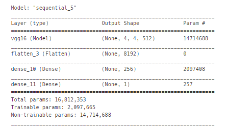
- block2_conv1 층 까지만 학습이 되도록 미세조정
# VGG16 모델 전체가 학습이 되도록 설저
conv_base.trainable = True

set_trainable = False

# VGG16의 신경망층 한 층을 가져온다
for layer in conv_base.layers:
    # 가져온 층의 이름이 block5_conv1이라면
    if layer.name == 'block5_conv1':
        set_trainable = True

    if set_trainable ==True:
        layer.trainable = True
    else:
        layer.trainable = False
- 미세조정 후 컴파일, 학습시키기
model5.compile(loss='binary_crossentropy',
              optimizer = 'adam',
              metrics = ['Accuracy'])
h5 = model5.fit_generator(generator = train_generator,
steps_per_epoch = 40,
epochs = 20,
validation_data = test_generator,
validation_steps = 20)import matplotlib.pyplot as plt
acc = h5.history['Accuracy']
val_acc = h5.history['val_Accuracy']
epoch = range(1, len(acc)+1)
plt.plot(epoch, acc, c='red', label = 'Train acc')
plt.plot(epoch, val_acc, c ='blue', label='Test acc')
plt.legend()
광주인공지능학원의 명훈쌤의 강의 덕에 CNN 개념은 확실하게 잡힌 것 같아요!
위 수업은 광주인공지능학원 에서 진행되었습니다.
광주인공지능학원 스마트인재개발원이 궁금하다면 아래 링크를 클릭하세요 !!
'+ 스마트인재개발원 +' 카테고리의 다른 글
| [광주인공지능학원] 딥러닝 과대적합 제어 (1) | 2021.08.09 |
|---|---|
| [광주인공지능학원] 딥러닝 활성화 함수 (1) | 2021.08.01 |
| [광주인공지능학원] 딥러닝 손글씨 분류하기 (1) | 2021.07.29 |
| [광주 인공지능학원] 딥러닝 개요 (1) | 2021.07.26 |
| [광주 인공지능학원] 안드로이드 Activity & Intent (1) | 2021.07.26 |


