| 일 | 월 | 화 | 수 | 목 | 금 | 토 |
|---|---|---|---|---|---|---|
| 1 | 2 | 3 | 4 | 5 | ||
| 6 | 7 | 8 | 9 | 10 | 11 | 12 |
| 13 | 14 | 15 | 16 | 17 | 18 | 19 |
| 20 | 21 | 22 | 23 | 24 | 25 | 26 |
| 27 | 28 | 29 | 30 |
- DataFrame
- iris붓꽃
- 인공지능학원
- 파이썬
- 데이터프레임
- python
- relu
- CountVectorizer
- 웹크롤링
- 스마트인재개발원
- 셀리니움
- jsp
- tfidf
- Selenium
- 자바
- 과대적합제어
- 광주인공지능학원
- 과대적합
- 유투브크롤링
- 딥러닝
- 인공지능
- 댓글분석
- 활성화함수
- servlet
- 토큰화
- sellenium
- permisision부여
- 머신러닝
- 크롤링
- 광주국비지원학원
- Today
- Total
+ Hello +
[광주인공지능학원] 딥러닝 손글씨 분류하기 본문
1. 손글씨 데이터 로딩
- datatset 불러오기
from tensorflow.keras.datasets import mnist- tensorflow는 튜플 형태로 받아와야함
((X_train, y_train), (X_test, y_test)) = mnist.load_data()

X_train.shape, y_train.shape
- 6000 : 데이터수
- 28 * 28 사진 데이터
2. 데이터 확인
import matplotlib.pyplot as plt

plt.imshow(X_train[0], cmap=plt.cm.binary)
- cmap=plt.cm.binary => 색상을 흑백으로 나타냄
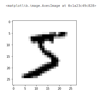
X_train[0]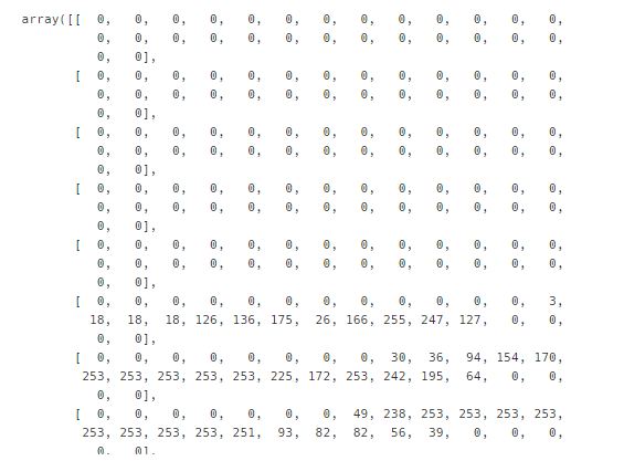
- 0~255까지의 숫자로 이루어짐
- 0이 흰색 / 255가 검은색
X_train = X_train.astype('float32') / 255
X_test = X_test.astype('float32') / 255
- 기계는 0과 1사이의 숫자를 좋아함
- 0~255까지의 숫자를 0~1까지로 만들어줌
- 전체 데이터를 255로 나누어줌
X_train = X_train.reshape((60000,28*28))
X_test = X_test.reshape((10000, 784))
- ((60000, 28, 28), (60000,))
- 28 * 28의 2차원 데이터를 784의 1차원 데이터로 만들어줄 필요가 있음
- input_dim에 집어넣기 위해서 ! -> reshape
X_train[0].shape
import numpy as np
np.unique(y_train)
- 출력층의 갯수 : 10
# 입력층 개수 : 784 (특성 데이터)
# 출력층 개수 : 10
import pandas as pd
y_train = pd.get_dummies(y_train)
y_test = pd.get_dummies(y_test)

import tensorflow as tf
seed = 100
np.random.seed(seed)
tf.random.set_seed(seed)
3. 모델설계
- 입력층, 중간층의 활성함수 : sigmoid
- 출력층의 활성화함수 : softmax
# 신경망 설계
from tensorflow.keras import Sequential
from tensorflow.keras.layers import Dense
model1 = Sequential()

# 입력층
model1.add(Dense(units=10, input_dim = 784, activation = 'sigmoid'))

# 중간층
model1.add(Dense(units=32, activation = 'sigmoid'))
model1.add(Dense(units=64, activation = 'sigmoid'))
model1.add(Dense(units=128, activation = 'sigmoid'))
model1.add(Dense(units=64, activation = 'sigmoid'))
model1.add(Dense(units=32, activation = 'sigmoid'))

# 출력층
model1.add(Dense(units=10, activation = 'softmax'))

model1.summary()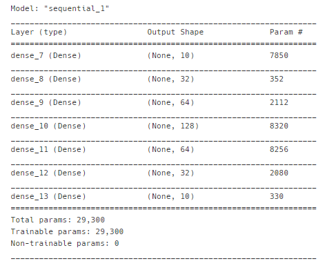
4. 모델 학습
model1.compile(loss = 'categorical_crossentropy',
             optimizer = 'adam',
             metrics=['accuracy'])
# 모델 학습 방법 설정
- loss : categorical_crossentropy
- optimizer : 'adam'
- metrics : accuracy
#  epochs = 20
history1 = model1.fit(X_train, y_train, epochs=20)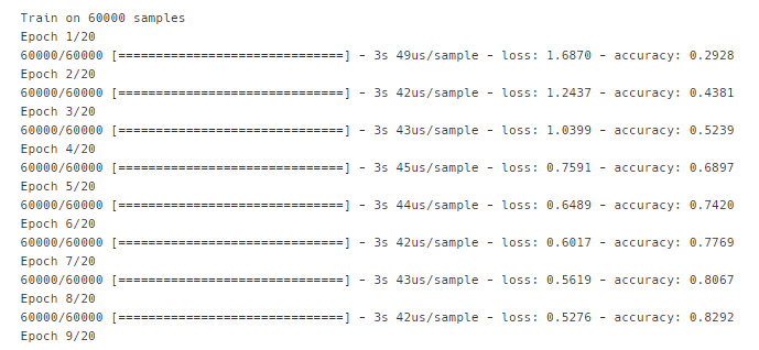
5. 모델 평가
model1.evaluate(X_test,y_test)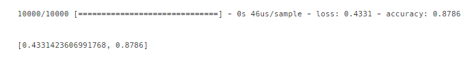
3-1) 활성함수 바꿔서 모델 설계
model2 = Sequential()
# 입력층
model2.add(Dense(units=10, input_dim = 784, activation = 'relu'))
# 중간층
model2.add(Dense(units=32, activation = 'relu'))
model2.add(Dense(units=64, activation = 'relu'))
model2.add(Dense(units=128, activation = 'relu'))
model2.add(Dense(units=64, activation = 'relu'))
model2.add(Dense(units=32, activation = 'relu'))
# 출력층
model2.add(Dense(units=10, activation = 'softmax'))
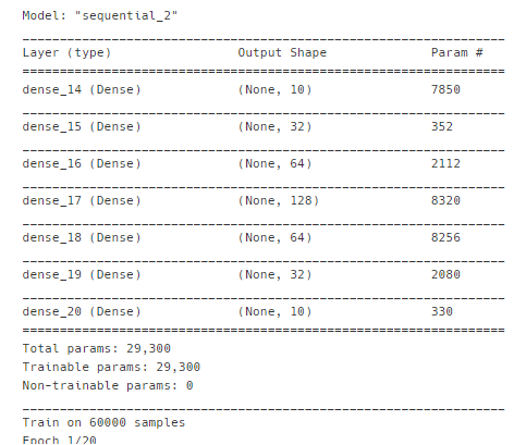
model2.summary()
model2.compile(loss = 'categorical_crossentropy',
optimizer = 'adam',
metrics=['accuracy'])
history2 =model2.fit(X_train, y_train, epochs=20)
model2.evaluate(X_test,y_test)- 모든 조건은 동일
- model2라는 딥러닝 모델 설계
- 입력층과 중간층의 활성화함수 sigmoid -> relu
- history2 = model2.fit()
5-1 ) 모델 평가
model2.evaluate(X_test,y_test)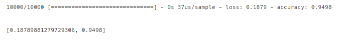
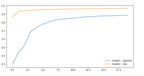
# model1 : 입력층, 중간층, 활성화함수 : sigmoid -> 결과값 : history1
# model2 : 입력층, 중간층, 활성화함수 : relu -> 결과값 : history2
plt.figure(figsize=(10,5))
plt.plot(range(20), history1.history['accuracy'],label = 'model1 - sigmoid')
plt.plot(range(20), history2.history['accuracy'],label = 'model2 - relu')

plt.legend() # 범례표시
plt.show()
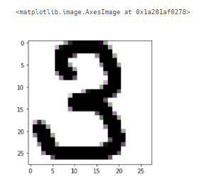
6. 직접 그린 그림 불러오기
import PIL.Image as pimg1) 3 그림 예측해보기
img_num3 = pimg.open('num_3.gif') # 내가 그린 이미지 저장
plt.imshow(img_num3)
- 이미지 확인 .imshow
img_num32) 손글씨 파일을 test 데이터로 만들어서 평가해보기
- 28*28 2차원 데이터 -> 784의 1차원 데이터로 변환
- 0~255의 픽셀값 -> 0 ~ 1사이의 픽셀값
3) 이미지 타입을 넘파이 배열로 변환
num3 = np.array(img_num3)
num3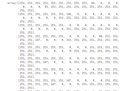
- 기존에는 흰색 : 0, 검은색 : 255에 가까움
# num3는 흰색 : 255, 흰색 : 0에 가까움 => 뒤집어주어야함
num3 = 255 - num3
3) 2 -> 1차원 데이터로 변환
- 0~255 -> 0~1의 픽셀로 변환
num3 = num3.reshape(1,784)
num3 = num3.astype('float32')/255
4) 예측하기
model2.predict(num3) * 100).astype('int')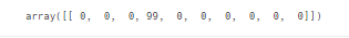
array([[ 0, 0, 0, 100, 0, 0, 0, 0, 0, 0]])
- 10개의 값이 출력됨
- 0 : 0%
- 1 : 0%
- 2 : 0%
- 3 : 100%
- ... 0%
model2.predict_classes(num3)- class 이름으로 알려줌
- array([3], dtype=int64) => 3이라고 100% 예측함
위 과정은 스마트인재개발원 수업 내용입니다.
'+ 스마트인재개발원 +' 카테고리의 다른 글
| [광주인공지능학원] 딥러닝 과대적합 제어 (1) | 2021.08.09 |
|---|---|
| [광주인공지능학원] 딥러닝 활성화 함수 (1) | 2021.08.01 |
| [광주 인공지능학원] 딥러닝 개요 (1) | 2021.07.26 |
| [광주 인공지능학원] 안드로이드 Activity & Intent (1) | 2021.07.26 |
| [광주인공지능학원] 스마트인재개발원 인공지능 과정 후기 (1) | 2021.07.19 |


